 Unexpected errors while looking for the best angular fit between the imaged stars and their reference locations.
My early efforts to map the imaged stars onto their virtual camera positions showed unexpected errors. They were close, but displayed error amounts that were inconsistent with a simple scale or rotation mismatch.
It seemed possible that the errors came about because of the radial distortion of the lens, which one reference suggested might be as much as 0.05%, a huge amount for this measurement.
To calibrate, a frame with more stars included (via increasing the ISO) were compared with their target (reference) locations and the radial errors were plotted and a correction curve computed to best fit them.
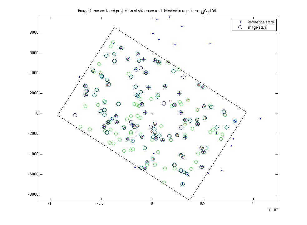 Reference stars and detected stars. The correlated pairs are used for evaluating radial distortion.
There are reference stars that do not have a corresponding star in the image, but there are many more detected stars without a reference coordinate. These may be spurious noise, or faint stars that were not listed in the reference star database (displayed by Stellarium).
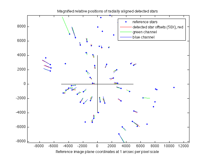 The correlated pairs of reference and detected image stars with an indication of the position discrepancies. Near-center stars are too close, and farther stars are too far.
The errors range over +/- 15 arcseconds, a few pixels in the image, but ten times the amount of deflection signal we are trying to detect.
To improve on this, we need to perform the rigid transform that finds the image center and angle that best aligns the detected stars with their reference locations.
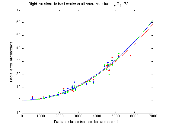 The radial errors, plotted as a function of distance from frame center. A polynomial fit is made to approximate them.
A radial correction function can then be obtained by finding a polynomial fit to the residual errors. This means that a function with factors of radius: r0, r1, r2, r3 etc. is used to approximate the distortion introduced by the lens. Knowing the distance from the center, we can use it to compute how the lens has shifted the star positions toward or away from the center, and then correct them.
I experimented with several forms of the polynomial function and found that the best behaved was among the simplest. It did NOT include an offset term (r0), and the linear term (r1, equivalent to magnification), was minimized by adjusting the overall base image magnification (arcseconds per pixel). This results in the linear term representing the slight differences in magnification between red, green and blue channels, something that apochromatic lenses strive to match but cannot be perfect at. The remaining error was well represented by the r2 term.
Here are the results averaged from multiple image frames of the eclipse target area:
Camera base magnification to reference frame (arcseconds per pixel):
scale = 2.8443; % average of EOS 6D calibration frames taken 20170601
This value is used in imagePos.m (step EE-2) as the scale factor to bring star positions into the reference frame where one increment (pixel) equals one arcsecond.
Linear (r1) coefficients (x10-3):
R 0.7731
G 0.5185
B 1.0245
Squared (r2) coefficients (x10-3)
R 1.1969
G 1.2564
B 1.1745
The linear coefficients are the differential magnifications between the red, green, and blue channels of the image. Green has a small (1/2 arcsecond per thousand) magnification difference from the base magnification. Red is a little higher, and the blue correction is about twice that of the green channel. The image would show a star’s image as having a green fringe toward the image center and a blue fringe at the outside. This captures the general chromatic aberration of the Televue-85 telescope I am using. It is a highly corrected lens that offers beautiful visual views; only a high resolution camera can quantify its color mismatch.
The squared coefficients indicate a general behavior of lenses and how ideal they are in projecting their field of view onto the perfect geometric projection we are using as our reference frame. These corrections are also quite small, but over enough radial distance contribute a position error that builds up to many arcseconds.
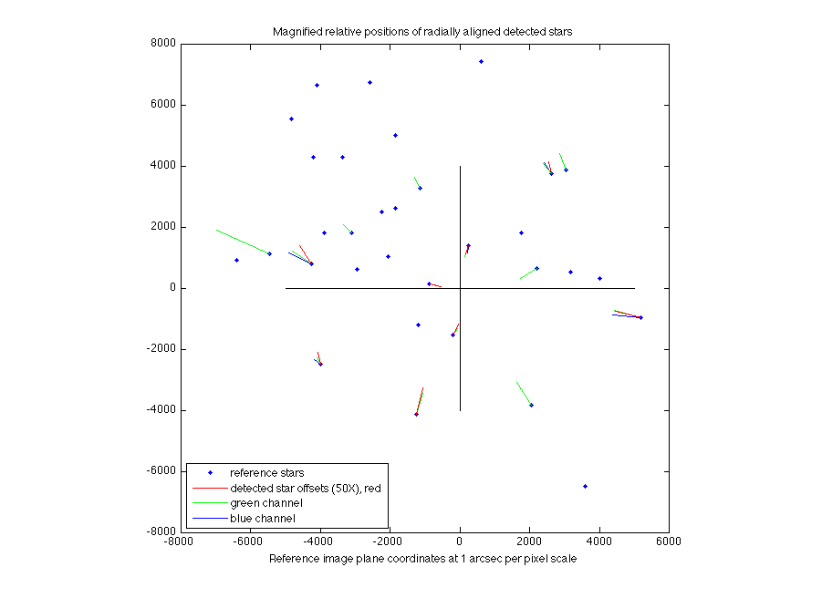
The lens correction coefficients (the linear and squared terms just described) are applied in step 3, radialAlign.m which provides the final set of detected star positions which have been angularly centered, and radial lens corrected. There are still some errors from the reference positions, but they are much reduced.
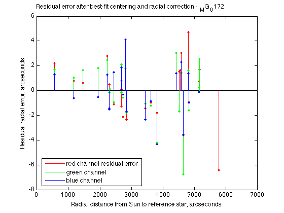
The remaining errors, plotted against radial distance from the center are limited to around +/- 5 arcseconds, and do not show any significant trend. If they did, we could identify it and apply additional corrections to remove it.
The residual errors after using the polynomial correction.
The radial correction brings the RMS errors to within 2 arcseconds (red) to 4 arcsec (blue). I’m not sure what the source of this residual error is, but it is of the same magnitude as typical Minnesota astronomical seeing. It may just be the twinkling motion of the stars. We could check this by comparing two separate exposures to see if the errors are correlated. If they are, then it is NOT due to atmospheric turbulence. If they are uncorrelated, then we need to find some way to overcome this variation, because it is larger than the signal we are looking for.

